

Statistics Overview
Statistics is the part of mathematics that deals with the accumulated information about a data collection. Usually, the collection characteristics cannot be described by an analytical formula because it is generated with or has an unreasonable volume of random processes.
Although prices usually do not follow it, short-term price action can be approximated to a Gaussian or Normal Distribution.
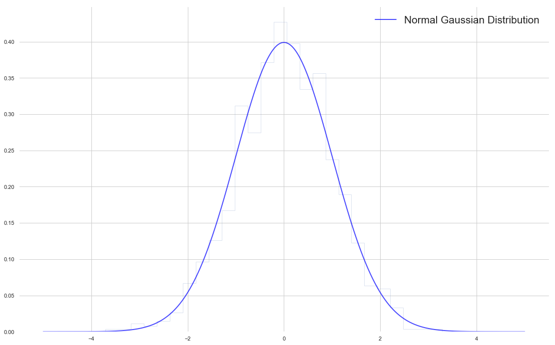
Fig 1 - The Normal Gaussian Distribution- Image Created using Matplotlib
This popular distribution can be described entirely by two measures: The centre and the variability off that centre.
On a Normal Distribution, the centre of is found by taking its mean.
Mean: The average of the data collection. It’s measured adding all the elements of the set and divide by its number:
Mean = Sum(p0-Pn-1)/n
The variability of a data set may be computed using a handful of methods. Two main ways are used in financial markets are:
The Range: The range is the most straightforward way to measure the variability. Is the distance between the highest and lowest points in a data set. Usually, on financial data, a variant of the range is calculated: The Average True Range, which delivers the average range over a time interval of the movement of prices.
Sample Variance(Var): Variance is a measure of the average distance of the data points around its mean. It’s measured by, first subtracting the mean from all points: (xi-mean) and squaring it. Then added together and dividing by n-1.
Var = 𝝈2 = 1/(n-1) x ∑ (x-mean)2,
where ∑ represents the sum of all members of the set next to it.
On this article, we are going to analyse a strategy based on the volatility changes as measured by the Average True Range. Concretely, we are going to use the Average True Range indicator to spot volatility sudden changes.
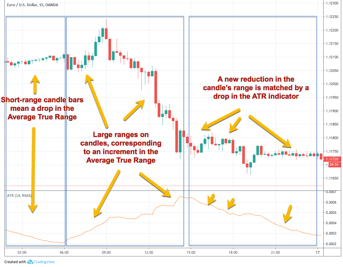
Fig 1 - The Average True Range in relation to Candlestick Lengths on the EURUSD 15M. Chart taken using TradingView.com. Click to enlarge
The concept
The concept of this strategy is for the market to tell which direction is going to head to. The premise is that an increase in volatility also will show the future market direction for a while. Therefore we always set two entry orders: A buy and sell stop orders at the open price on every bar plus and minus a multiple of the Average True Range of the last few bars.
If the price reaches that value on the long side it means volatility has expanded and the trend is bullish. If it catches the short order it went into the bearish side.
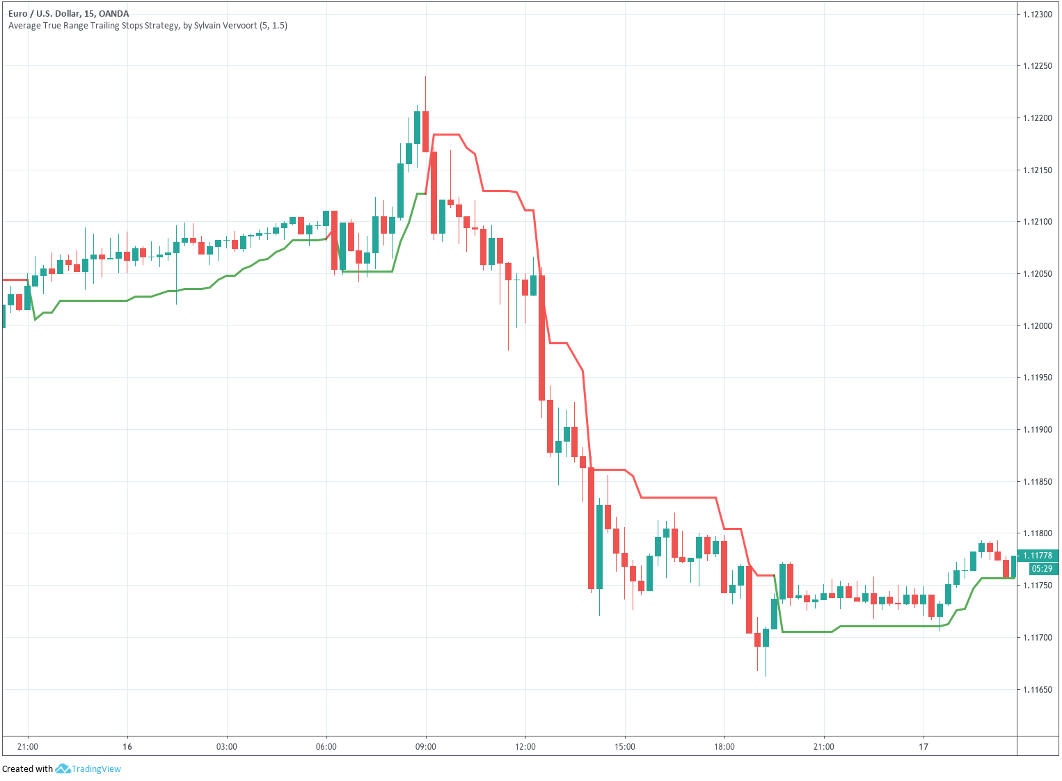
Fig 2 - A Volatility Strategy using 1.5x ATR on the EURUSD 15M. Chart taken using TradingView.com. Click to enlarge
The rules of the strategy are:
Long Entries:
Set a buy stop order at Open + Average( Range, Length) * NumRanges next bar
Short Entries:
Set a stop sell short order at Open - Average( Range, Length ) * NumRanges next bar
Explanation
A Stop Order is a delayed entry order that is placed at a price above the current price, if long, or below it, if short. That means the order is activated only if the price moves from the current level in the direction forecasted by the stop order and touches the stop level.
The parameters are the Length of the average and the NumRanges for longs and shorts.
The trade is managed using a trailing stop.
Let’s see how an un-optimized system performs under 14 years of EURUSD hourly data:
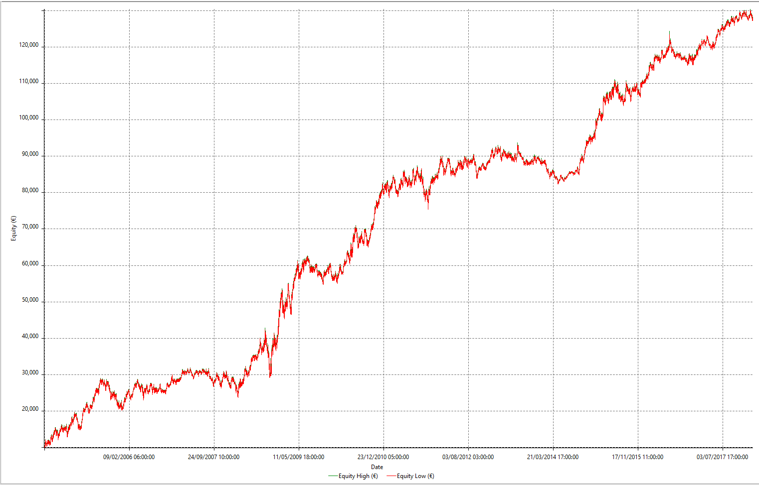
Fig 3 - Un-optimised Volatility Expansion Strategy Equity Curve
The standard parameters are:
   Length: 4
NumRanges: 1.5
As we can observe, the actual raw curve is rather good, showing a continuously growing equity balance; and, although we find difficult moments, the long-term strategy has an edge.
The Total Trade Analysis for single-contract trades shows a nice 2:1 Reward to risk ratio (Ratio Avg Win/Avg Loss) although just a 35% winners.
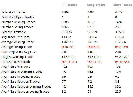
Fig 4 - Total Analysis Table of the Standard Volatility Expansion Strategy
Analysing the Parameter map:
To optimise this strategy we created two optimisation 3D maps to show the relevance of the two parameters: ATR length and ATR multiplier in the long and short trades.
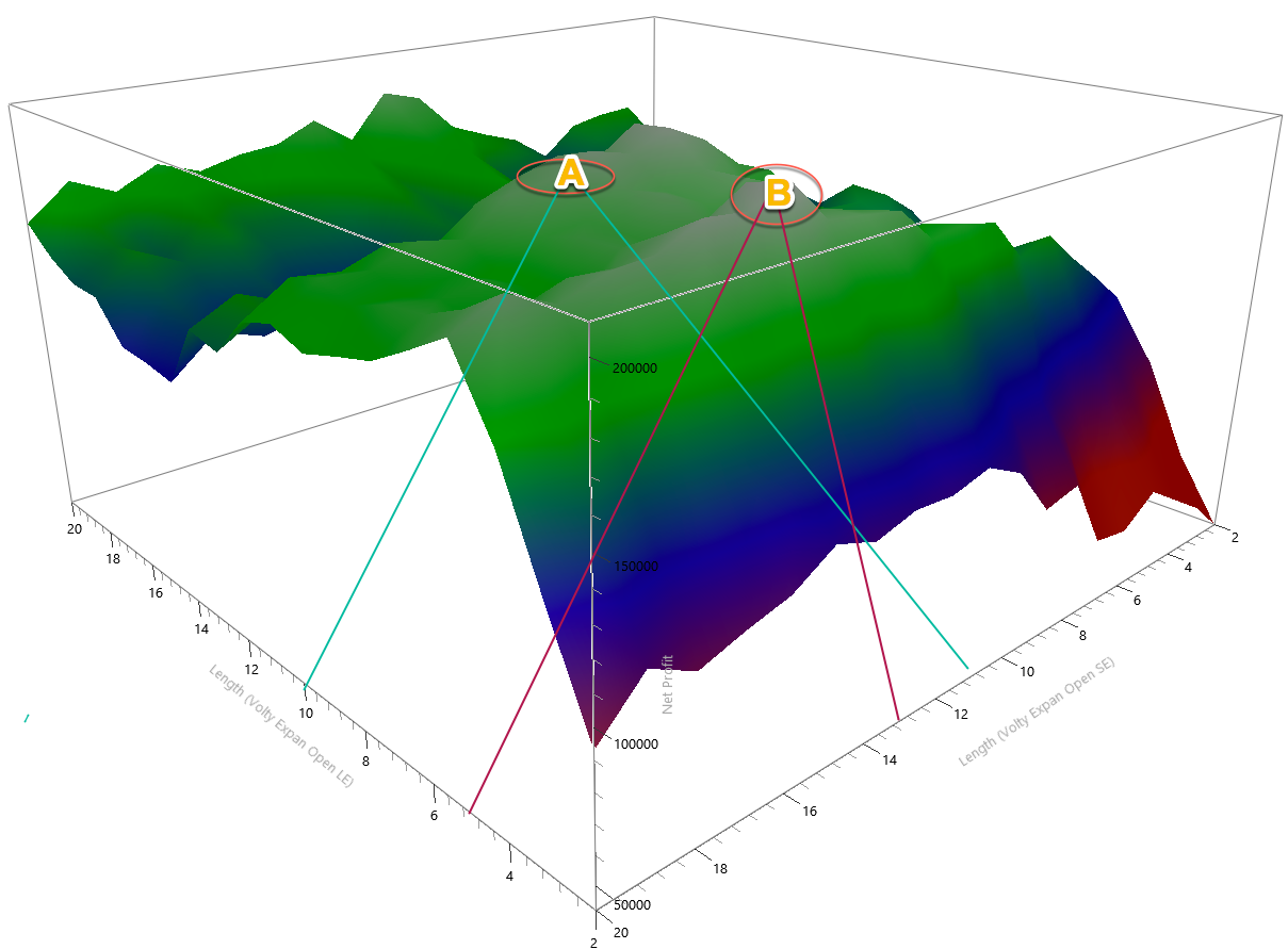
Fig 5 - ATR Length Parameter Map
As we observe in fig 5, there are two areas A and B where to locate the best parameters for this strategy. The surface is smooth, thus, guaranteeing that a shift in market conditions won’t harm too much the strategy. For the sake of symmetry, we will choose the A region. Thus, the Long ATR length will be 10, and the short ATR length is left at 13.
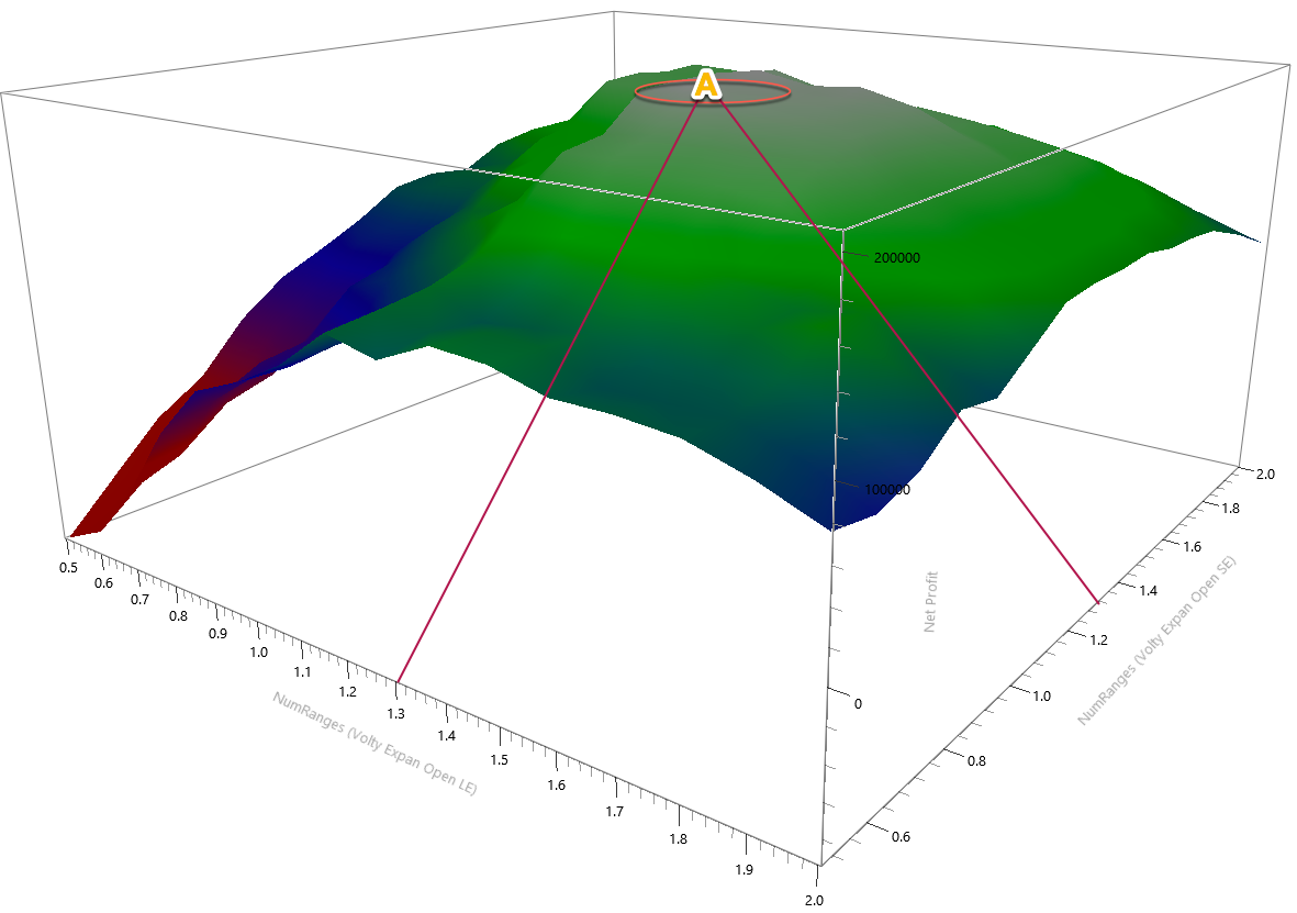
Fig 5 - ATR Multiplier Parameter Map
Fig 6 shows the map for the NumRanges That multiplies the ATR value to set the distance of the stop order from the current open. The surface is, also, very smooth. Therefore we can be relatively sure that setting the NumRages value to 1.3 in both cases we will get good results.
The new equity curve has improved a lot, especially in the drawdown aspect, and in the overall results, as well, although we know this isn’t a key aspect because this equity result was achieved with just a single-contract trade. This is the best way to evaluate any strategy, separating the normalised result from the position sizing decision.
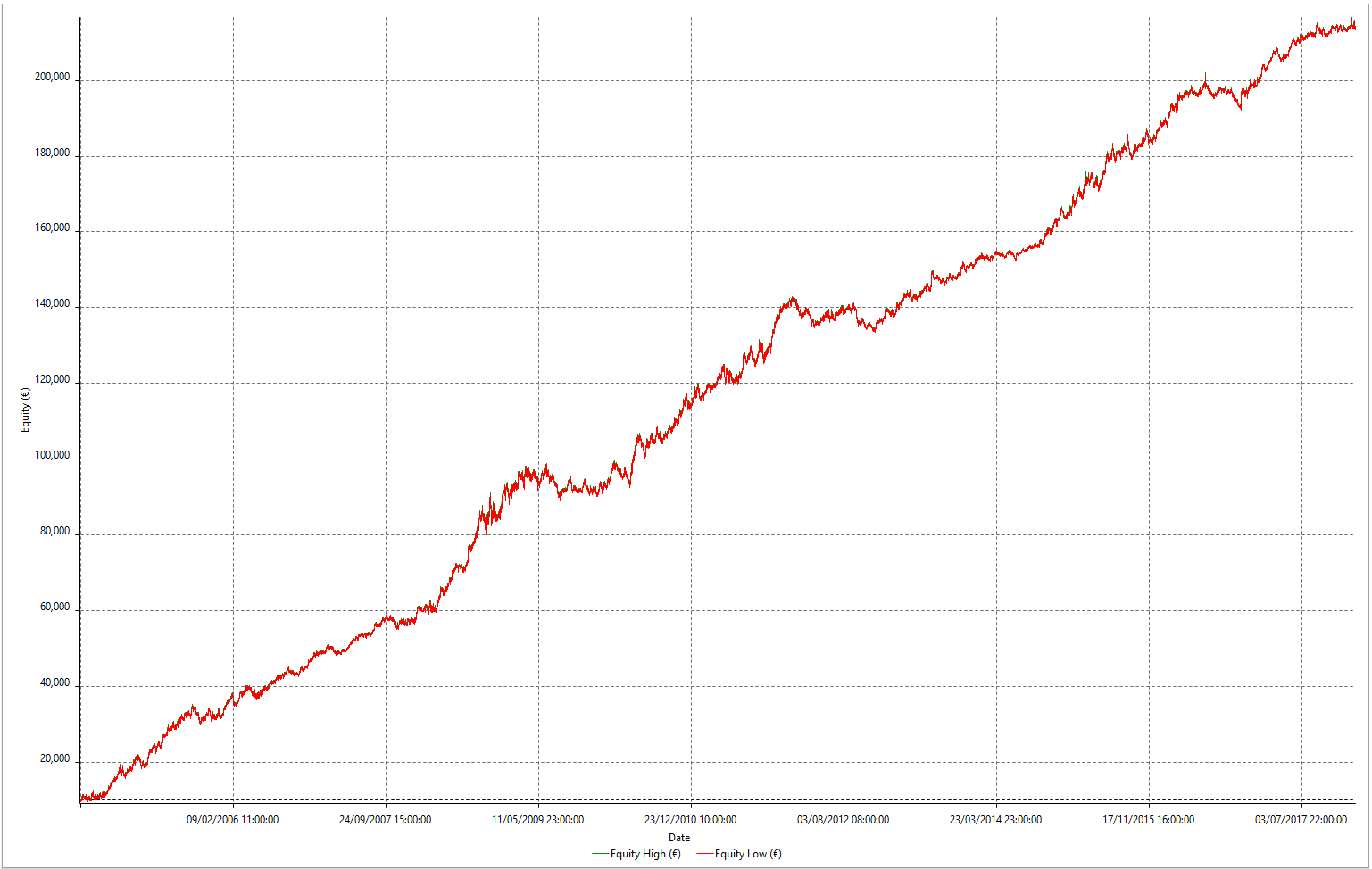
Fig 7 - Optimised Volatility Analysis Strategy in 14 years of the EURUSD pair
This kind of strategy incorporates its stops because it’s a reversal system. Therefore there is no need for further stops or targets.
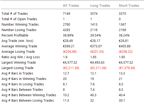
On fig 8, we observe that the per cent winners grew to 39% while the risk to reward ratio represented by the ratio Avg win/ Avg loss is 1.9. Also, we see that the average trade jumped from 13.32 to 28.5 euros, which is a huge jump in the money expected to gain on every trade. That shows robustness and edge.
Conclusions
We can see that when applied in it’s standard and unoptimised version to 14+ years of EURUSD data using 1-hour charts, the Volatility Expansion Strategy has performed quite well. The system is rather simple. Just two parameters and there is no stop loss or take profit.
The robustness of the Volatility Expansion strategy is further confirmed when we plot the parameter maps and see round and flat surfaces. That means a change in market conditions will not affect catastrophically the performance of this volatility.
The optimised strategy performs excellently with reward-to-risk ratios of 1.9 and close to 40% winners. That is really fantastic for a two-parameter strategy.
As an after-thought, we could estimate convenient a kind of weekly or monthly parameter optimisation to keep this system in tune with the market conditions and further improve its performance.
The images of the strategy analysis, including parameter maps equity curves and performance tables, were created with Multicharts 12 (TM) Platform.
