Wave Projection Forecasts Using Cynthia Kase’s Methods

It’s tough to make predictions, especially about the future.

Yogi Berra

Cynthia Kase and Forecasting

This is our second article in which we discuss Cynthia Kase’s excellent forecasting ideas and methods. This article has been extracted from chapter 3 of his book Trading With The Odds, published in 1996.

No trader has a crystal ball, but forecasting is not about predicting the future. For a professional trader, it means creating potential scenarios to make flawless trading plans. Traders commiting themselves to this kind of exercise, together with proper money management, will have a clear edge against the rest of the trading crowd, only looking to scalp the fast and easy trade.

The Elliott Wave as a Forecasting Tool

Kase’s primary forecasting method is the use of the Elliott Wave theory along with Fibonacci retracements and extensions.

The key idea when using the Elliott Wave theory to trade is preparation during corrective segments to be ready to trade the next impulsive segment. To accomplish it, the trader needs to perform three tasks:

1.- Count waves to determine where in the wave map is the current price action

2.- Plan for an entry point on the breakout of the current corrective structure

3.- Forecast the potential targets by analysing possible endings of the next impulse.

The last part is the more tedious part as it should find confluences between various results to reach a conclusion about the most probable target level. When several methods of analysis come to similar results, the degree of confidence in the scenario grows.

Review of the Wave patterns

The basic pattern is an impulse followed by a correction. This impulse, as we know, is composed of five waves, three impulses and two corrections. Finally, the corrective segment is composed of three sub-waves, two impulsive and one corrective.

These rules were developed for the stock market indices and not always applies to commodities or forex pairs since a forex pair does not have any inherent bullish bias. The trader has to analyse the current behaviour of the pair to assess if it is necessary to apply any modification to the theory to match what the market does.

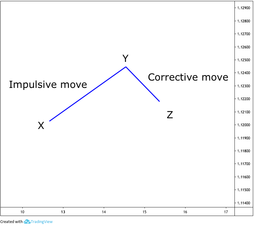
Fig 1 - Idealised Elliott waves

The basic guidelines given by Elliott were:

1.- Wave 3 never is the smallest Wave.

2.- Wave 3 usually is the largest Wave, except when there is an extended Wave 5

3.- Two of the waves are usually of the same size.

As a corollary: If any of the impulsive waves are extended, the other two impulses are of similar size.

The alternation rule also says that if Wave 2 is complex, Wave four will be simple and vice versa.

Chart continuation formations such as flags, pennants, wedges and the like are complex Elliott structures. These structures are tough to trade, so it is not worth the effort. Better is to wait for a breakout to jump into the next impulsive Wave.

Finally, we should remember that the fractal structure of the market tells that every Wave is composed of smaller waves of a lesser degree.

The Numerical Formulation

Cynthia Kase uses three classes of formulae to forecast the markets: Extensions, projections from retracements and the “rule of three”.

The figure below illustrates the Kase conceptual scenario. We have named X, Y and Z points as she originally did.

The impulse move goes from X to Y and its correction from Y to Z. All three forms the group XYZ.  This XYZ group will show inverted on bearish movements.

These points are not part of the naming conventions of the Elliott Wave analysis but a construct she uses to identify initial and end points of these structures.

Extensions To compute extensions, the price difference between X and Y is multiplied by three Fibonacci ratios. The results are, then projected from the Z point.

Note: The p besides the capital letters means price.

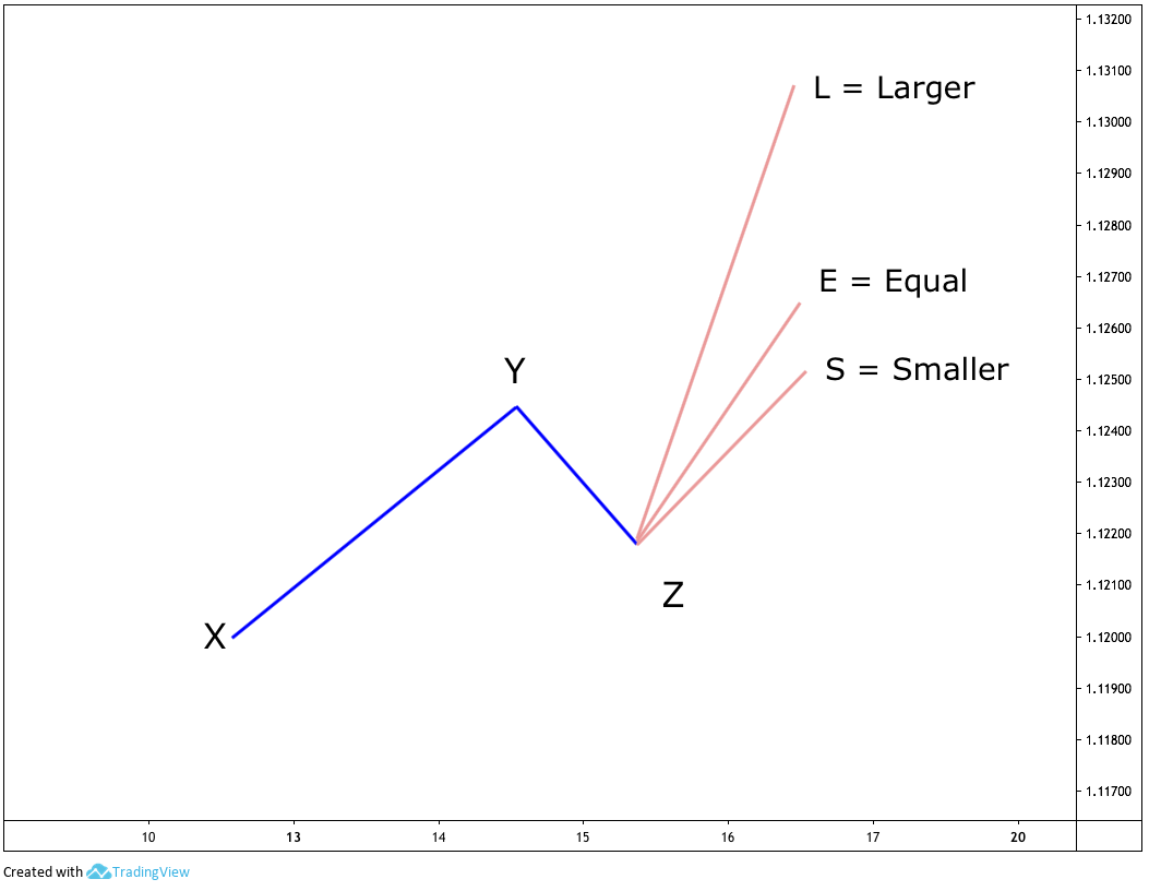
Fig 2 - Smaller, Equal and Larger than Rule projections

Projecting using Corrective Movements

Corrective movements are the price activity from Y to Z. Therefore, instead of looking for a price difference between initial and end points of the Wave 1, which is the length of Wave1, we look for differences in price between the beginning of Wave 2 and Wave 3, which is the price length of Wave 2.

She calls them:

IT (if it’s correcting a Third wave): Most of the time, this correction, which is Wave 4, will extend the next movement by 1.618 of its magnitude.

IF (If it is correcting the first wave): Miss Kase tells that most of the time this correction extend the correcting Wave (wave 2 of Wave 1 or Wave b correcting Wave a) by 1.618 squared.

 IX (if the market is correcting a first wave extended beyond IF), then the extension would go up to the correction size by 1.1618 cubed.

The Rule of Three

The Rule of Three is the most straightforward way to forecast a future ending wave. It multiplies Wave 1 size by three and adds it to, again, the beginning of Wave 1. Cynthia says in his book that since the market does not move linearly but exponential, it is needed that the price is reduced to log scale before adding it and then converted back.

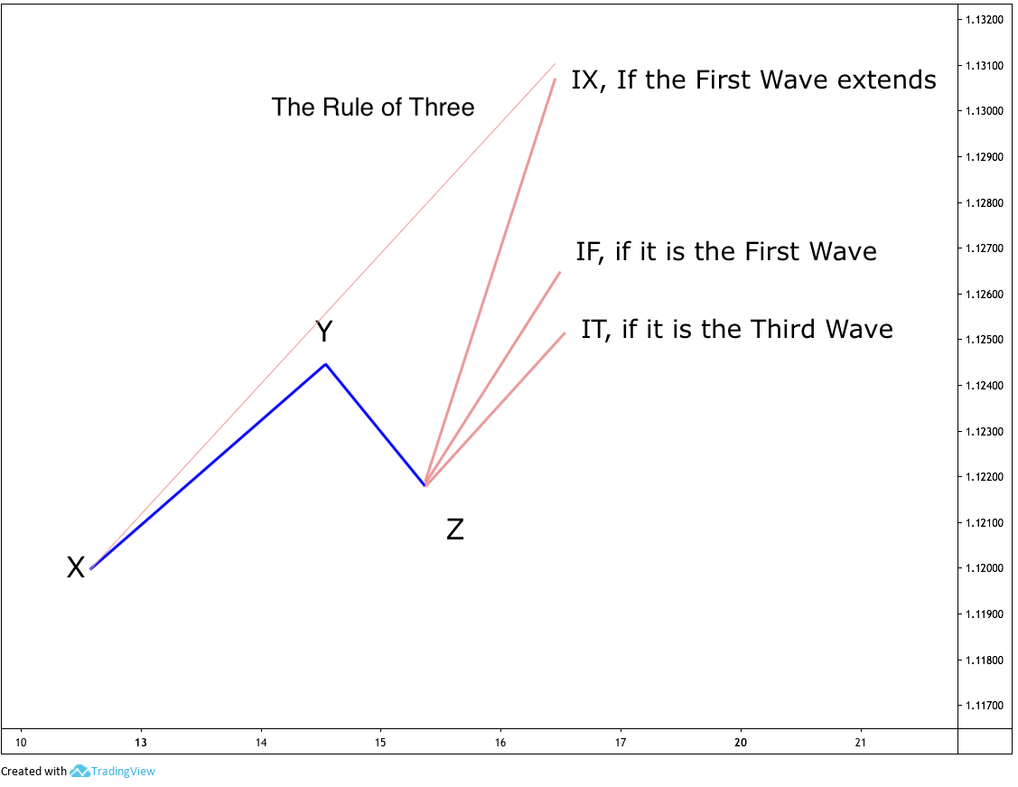
Fig 3 - Projection classes from a retracement

Applying the Rules

Once calculated all the possible ways the price could move, we need to decide about the most probable scenario of all.

Smaller than the Rule (Sp)

In a situation when Wave 1 and Wave 3 are complete, the trader is trying to predict Wave 5 length.  So, if for instance, Wave 2 and 3 are of similar length and relatively large, which would you think the length of Wave 5 would be? Wave 3 is never the shortest and tends to be the longest. Under this scenario, being Wave 1 of similar length, the expectation is for Wave 5 to be the shortest of the three impulses. Therefore, it could be used to arrive at the most probable price length for Wave 5.

Another moment when this rule can be used is if Wave 1 is close to 0.618 of Wave 3, being Wave 3 the largest Wave, we can think that the other two waves are of similar length, so Wave 5 would be equal to Wave 1.

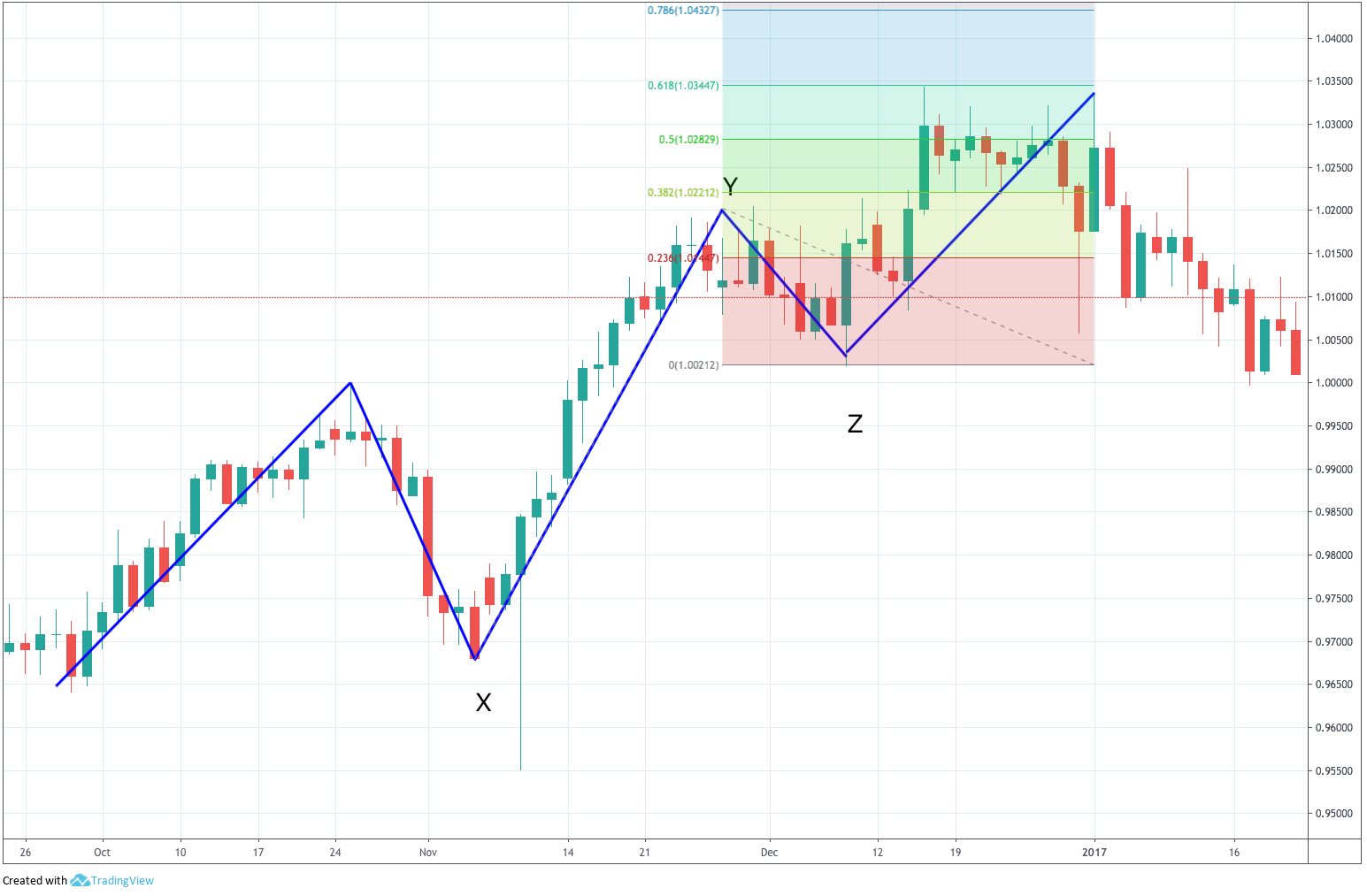
Fig 4 - Less than Rule Projection on a 5th Wave (click on it to magnify)

Equal to Rule

Here the author presents the example of the case of a very tiny wave 1 and a large wave 3. On this case, the probability of another tiny 5th wave is low, so the best path is to equate Wave 5 to wave 3 unless it becomes extended. This also applies to ABC corrections.

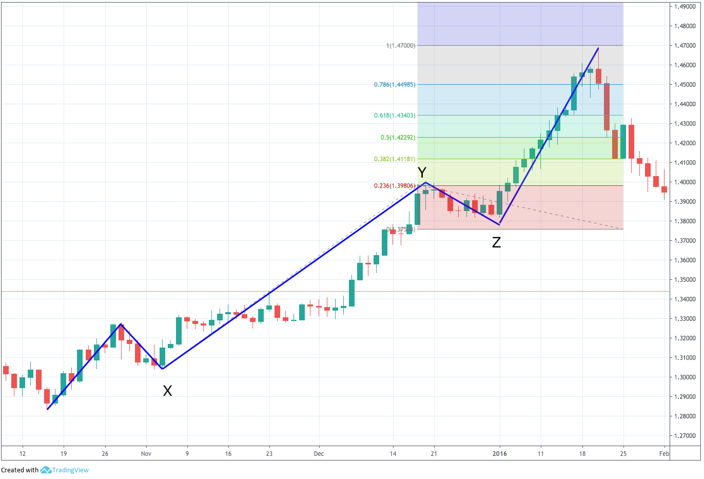
Fig 5 - Equal than Rule Projection on a 5th Wave (click on it to magnify)

Longer than Rule

If Wave 1 is complete and Wave 3 is still unfinished but already larger than Wave 1 and continues growing then the length of Wave 1 multiplied by 1.618 may forecast the end of Wave 3. This also works in corrective ABC structures.

Fig 6 - Longer than Rule Projection on a 3rd Wave (click on it to magnify)

IT, IF, and IX Rules

IT - If it is the Wave 3, or Wave c

IF - If it is the Wave 1, or Wave a

IX - If it is the Wave 1, or Wave a, extended

Mrs Kase recommends to calculate IT, IF and IX rules for the first and third wave corrections, and address specific situations ad they manifest themselves.

The Rule of Three

The Rule of Three can be used whenever a Wave 1 is detected. As said earlier, the logarithmic extension should be applied.

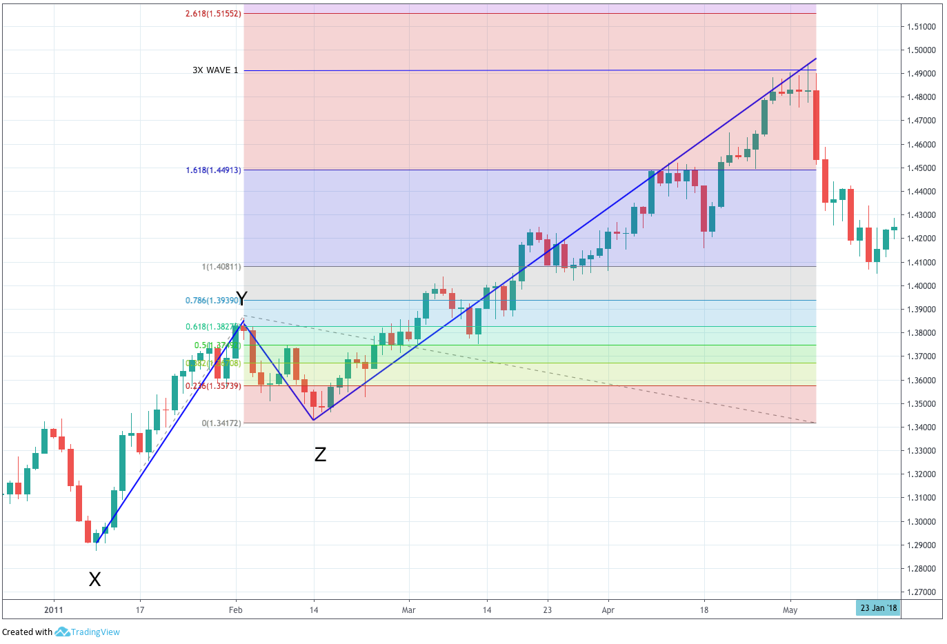
Fig 7 - The Rule of Three Projection on a 3rd Wave (click on it to magnify)

 

In a future article, we will discuss how to deal with retracements.

 

---

 

Reference: Trading With The Odds, Chapter 3. Cynthia Kase.

All graphs made using TradingView.com on line charting tools